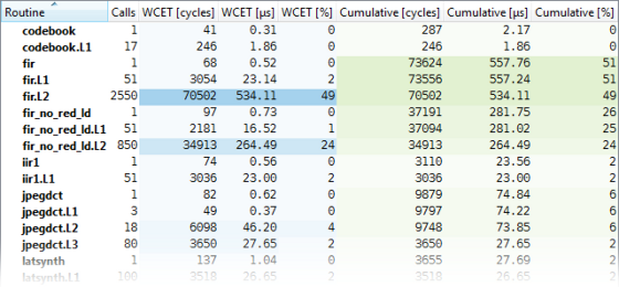
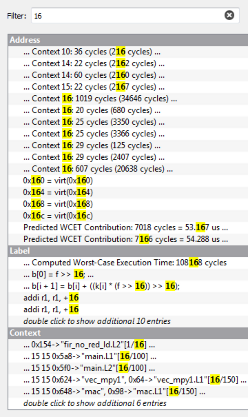
Filter options in Statistics views
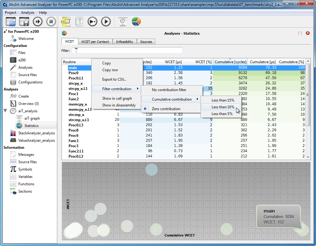
The routine list in the WCET tab and the tree view in the WCET per Context tab can now be filtered by cumulative contributions of routines. This is done from the context menu accessible by right-clicking. The following options are available:
- No contribution filter
- Less than 15%
- Less than 10%
- Less than 5%
- Zero contribution
The first option disables the filter, the others hide all routines with the specified cumulative contribution to the overall WCET. The default is hiding all routines with zero contribution.
Additionally, the tree map view in the WCET per Context tab no longer displays the WCET contributions for the entire program, but rather the cumulative contributions up to a specified call depth. The default depth is 1. It can be configured by right-clicking on the tree map and selecting one of the following options:
- No depth limit
- Depth 1
- Depth 2
- Depth 5
- Decrement by 1 (unless the current depth is 1)
- Increment by 1 (unless the current depth is infinite)
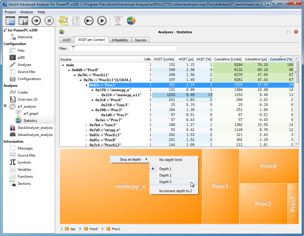
Example with a call depth of 1
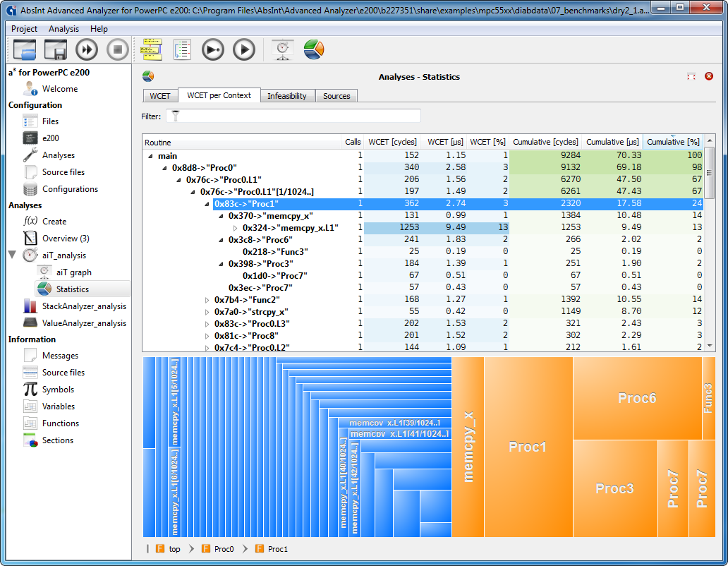
The same example with an infinite call depth
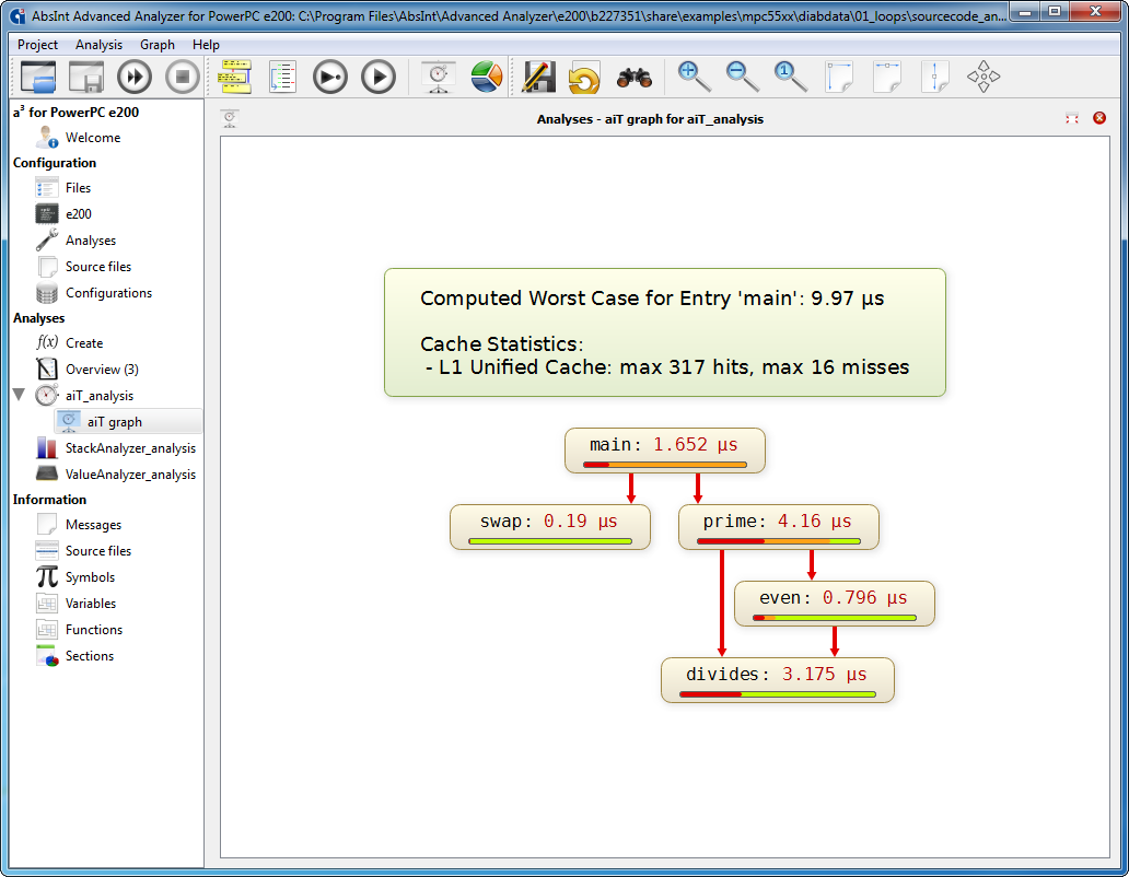
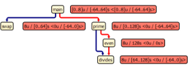
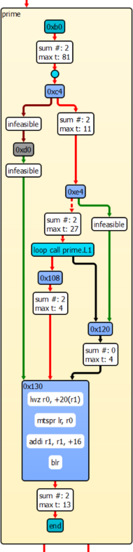
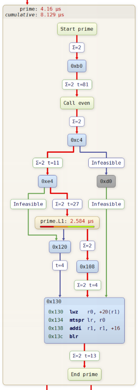
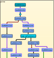
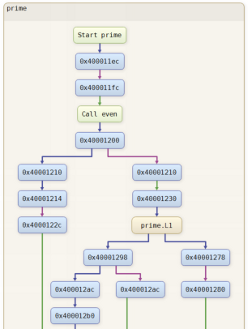
Improved call graphs
The pictures below offer a quick overview of the most important changes.
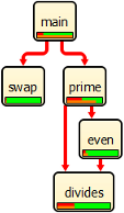
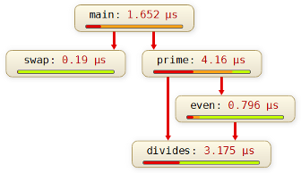
Fonts and colors have been made easier on the eye. In graphs resulting from timing analysis, routines are now directly labeled with their WCET. The cumulative-WCET bars have been simplified without losing information.
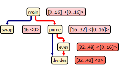
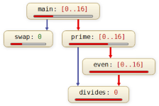
Likewise, in graphs resulting from stack analysis, routines are now directly labeled with their local stack usage. The global stack usage is now represented by colored bars, by analogy to WCET graphs. Exact figures are still available in additional information windows, the various Statistics views, and at the control-flow graph level.
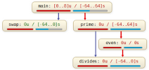
For targets with two or more stacks, each stack is visualized separately. The view is no longer cluttered with excessively long and complex strings of numbers.
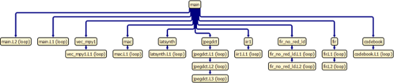
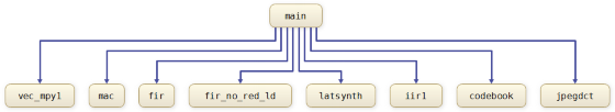
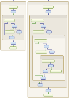
Loops are now always displayed inlined in their routines rather than being extracted into routines of their own. This results in less busy call graphs and a more intuitive visualization overall, especially for nested loops.
In WCET statistics tables and the like, loops are still listed separately, so you can still see at a glance how they contribute to the worst-case behavior.
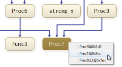
You can now quickly navigate from a routine to any of the locations it is called from, by selecting it and picking “Goto caller” from the context menu, or pressing C. (From there, you will also be able to navigate right back by using the complement operation “Goto target”, or pressing T.) This is especially useful for browsing large graphs with long edges.
Infeasible routines are still dark gray and backwards infeasible ones light gray.
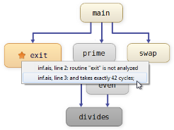
Not-analyzed routines are still orange. This includes virtual call-target and interrupt routines. Generally, orange routines do not contain code, while gray and yellowish routines do.
Just like in the Source Code view, AIS-annotated locations are now signified by orange stars that are linked to the annotations in the AIS file.
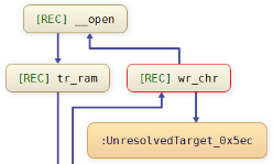
Recursive routines and routines that are part of recursion rings are marked with a “[REC]” before their names.
Routines with unresolved calls are marked by a red border. The unknown call targets are represented by orange virtual routines.
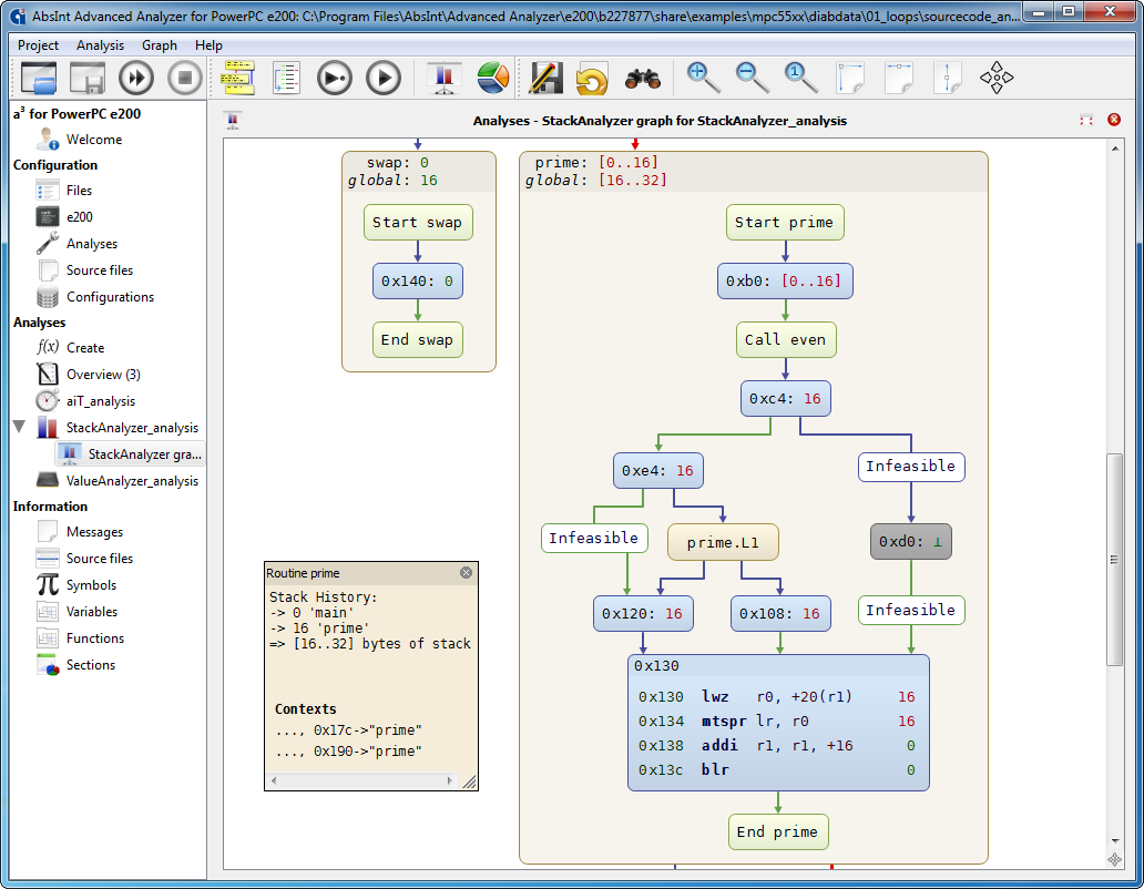
Improved control-flow graphs
The pictures below offer a quick overview of the most important changes.
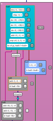
The color coding has been simplified:
- The default edge color is now the same as at the call-graph level.
- The red color is no longer overloaded. True edges after branches are still green, but false edges are no longer red. Only edges on WCET paths are red now, and dashed red edges are gone completely.
- Recursive routines no longer have a lilac background. This color, too, used to be overloaded and is now reserved for targets with delayed branch instructions.
- Within the basic blocks, instructions are now simply listed sequentially with the same background color as the block itself.
- The first basic block of a routine no longer has a special color, but is marked by a special node "Start routine name".
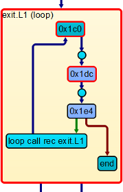
The end block now similarly features the routine’s name for easier orientation, and calls to other routines are likewise clearly labeled "Call routine name", rather than being represented by a nondescript circle. The call nodes are linked to their call targets via the new command “Goto target”, which can be invoked from the context menu or simply by selecting a call node and pressing T.
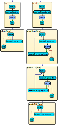
Loops are now always shown within their routines, rather than being extracted to dummy routines of their own. This provides for a more intuitive visualization and a less steep learning curve.
Just as before, the loop transformation only concerns the graphs; the executable itself is not affected or transformed in any way (as can be verified by checking the Disassembly view).
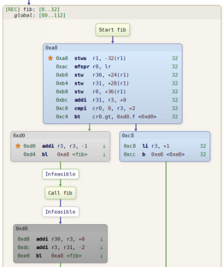
For each instruction, its address is now shown right next to it rather than being hidden in an additional information window. The instructions are also aligned and formatted in a much more readable manner. AIS-annotated instructions are marked by orange stars that are linked to the annotations in the AIS file.
Likewise, local and global analysis results of a routine have moved from its additional information window directly to its title bar.
There are now fewer additional information windows overall:
- A node can only carry at most one info window now, rather than up to three as before.
- Individual instructions no longer have any info windows at all.
The most useful info windows are now those of routines, WCET-analysis edge labels, and UCB-analyzed basic blocks for targets with this feature supported.
The graph viewer toolbar has been cleaned up as well, such that the three different info-window buttons are gone. The windows are still accessible from context menus as well as via the familiar shortcut I. When several windows are open, they can be toggled off and on again all at once, just like before, by using Shift+I.
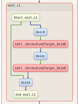
Unresolved calls are now marked in red themselves, rather than being indicated by a red border of the preceding basic block. Additionally, the calls are now labeled in a self-explanatory manner.
For targets with delayed branch instructions, the delay edges are still violet, but their target nodes no longer have a violet border.
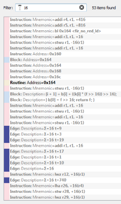
Search results are no longer grouped by type. Instead, the type is now stated for each result separately. Nodes and edges are now color-coded, just like in the graph itself. Navigating to a result in the graph works as before (click to center, double-click to center and unfold).
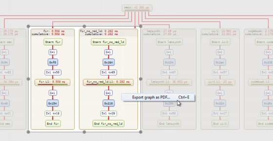
Any graph region can now be directly exported to PDF. Simply select any nodes or subgraphs and press E for an instant preview. If needed, use the mouse to fine-tune the selection. Then press Ctrl+E, or right-click to export the area from the context menu.